Pipe Fitting Losses
Head loss in a pipe is sum of following -
- Elevation difference, hZ
- Fitting losses, hL
- Friction losses, hF
Fitting losses hL is calculated as
hL = K(V²/2g)where, K is resistance coefficient due to fittings, V is fluid velocity and g is acceleration due to gravity.
Friction losses hF is calculated as
hF = f(L/D)(V²/2g)where, f is Darcy's pipe friction factor, L is pipe length and D is pipe inside diameter.
Total head loss in a pipe -
hTotal = hZ + hL + hFPressure drop due to head loss in pipe is calculated as
ΔP = hTotal.ρ.gwhere, ρ is fluid density.
There are several methods for estimating pipe fitting losses like equivalent length method, K method, 2-K (Hooper) method and 3-K (Darby) method. 3-K method is most accurate followed by 2-K method.
2-K (Hooper) Method
K = K1/Re + K∞ (1 + 1/ID )where, Re is Reynold's number, K1, K∞ are constants and ID is inside diameter in inches.
3-K (Darby) Method
K = K1/Re + K∞ (1 + Kd/Dn0.3 )where, K1, K∞, Kd are constants and Dn is nominal pipe diameter in inches.
Constants for 3K and 2K method for some common fittings.
| 90° Elbow | K1 | K∞ | Kd |
|---|---|---|---|
| Threaded, r/D = 1 | 800 | 0.14 | 4.0 |
| Threaded, Long Radius, r/D = 1.5 | 800 | 0.071 | 4.2 |
| Flanged, Welded, Bend, r/D = 1 | 800 | 0.091 | 4.0 |
| Flanged, Welded, Bend, r/D = 2 | 800 | 0.056 | 3.9 |
| Flanged, Welded, Bend, r/D = 4 | 800 | 0.066 | 3.9 |
| Flanged, Welded, Bend, r/D = 6 | 800 | 0.075 | 4.2 |
| Mitered, 1 Weld, 90° | 1000 | 0.270 | 4.0 |
| Mitered, 2 Weld, 45° | 800 | 0.068 | 4.1 |
| Mitered, 3 Weld, 30° | 800 | 0.035 | 4.2 |
| 2K Method | |||
| Mitered, 4 Weld, 22.5° | 800 | 0.27 | |
| Mitered, 5 Weld, 18° | 800 | 0.25 | |
| 45° Elbow | K1 | K∞ | Kd |
|---|---|---|---|
| Standard, r/D = 1 | 500 | 0.071 | 4.2 |
| Long Radius, r/D = 1.5 | 500 | 0.052 | 4.0 |
| Mitered, 1 Weld, 45° | 500 | 0.086 | 4.0 |
| Mitered, 2 Weld, 22.5° | 500 | 0.052 | 4.0 |
| 180° Bend | K1 | K∞ | Kd |
|---|---|---|---|
| Threaded, r/D = 1 | 1000 | 0.230 | 4.0 |
| Flanged/ Welded, r/D = 1 | 1000 | 0.120 | 4.0 |
| Long Radius, r/D = 1.5 | 1000 | 0.100 | 4.0 |
| Tees | K1 | K∞ | Kd |
|---|---|---|---|
| Standard, Threaded, r/D = 1 | 500 | 0.274 | 4.0 |
| Long Radius, Threaded, r/D = 1.5 | 800 | 0.140 | 4.0 |
| Standard, Flanged/ Welded, r/D = 1 | 800 | 0.280 | 4.0 |
| Stub-in Branch | 1000 | 0.340 | 4.0 |
| Run Through, Threaded, r/D = 1 | 200 | 0.091 | 4.0 |
| Run Through, Flanged/ Welded, r/D = 1 | 150 | 0.050 | 4.0 |
| Run Through Stub in Branch | 100 | 0 | 0 |
| Valves | K1 | K∞ | Kd |
|---|---|---|---|
| Angle Valve = 45°, β = 1 | 950 | 0.250 | 4.0 |
| Angle Valve = 90°, β = 1 | 1000 | 0.690 | 4.0 |
| Globe Valve, β = 1 | 1500 | 1.700 | 3.6 |
| Plug Valve, Branch Flow | 500 | 0.410 | 4.0 |
| Plug Valve, Straight Through | 300 | 0.084 | 3.9 |
| Plug Valve, 3-way, Flow Through | 300 | 0.140 | 4.0 |
| Gate Valve, β = 1 | 300 | 0.037 | 3.9 |
| Ball Valve, β = 1 | 300 | 0.017 | 3.5 |
| Butterfly Valve | 1000 | 0.690 | 4.9 |
| Swing Check Valve | 1500 | 0.460 | 4.0 |
| Lift Check Valve | 2000 | 2.850 | 3.8 |
| 2K Method | |||
| Diaphragm Valve, Dam Type | 1000 | 2.0 | |
| Tilting Disk Check Valve | 1000 | 0.5 | |
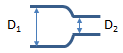
Square Reduction
For Re1 < 2500
K = (1.2 + 160/Re1)[(D1/D2)4 - 1]For Re1 > 2500
K = (0.6 + 0.48f1)(D1/D2)²[(D1/D2)² - 1]Re1 is upstream Reynold's number at D1 and f1 is friction factor at this Reynold's number.
Tapered Reduction
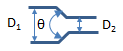
For θ < 45°, multiply K from square reduction by 1.6 sin(θ/2).
For θ > 45°, multiply K from square reduction by sin(θ/2)0.5.
Rounded Pipe Reduction
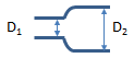
K = (0.1 + 50/Re1)[(D1/D2)4 - 1]Square Expansion
For Re1 < 4000
K = 2[1 - (D1/D2)4]For Re1 > 4000
K = (1 + 0.8f1)[1 - (D1/D2)²]²Re>Re1 is upstream Reynold's number at D1 and f1 is friction factor at this Reynold's number.
Tapered Expansion
For θ < 45° multiply K for square expansion by 2.6 sin(θ/2).
For θ > 45° use K for square expansion.
Rounded Pipe Expansion
Use K for square expansion.
Thin Sharp Orifice
For Re1 > 2500
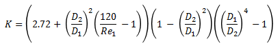
For Re1 > 2500
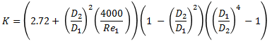
Thick Orifice
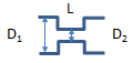
For L/D2 > 5, use equations for square reduction and a square expansion.
For L/D2 < 5, multiply K for a thin sharp orifice by
0.584 + (0.0936 / ( (L/D2)1.5 + 0.225))Pipe Entrances
Flush/ Square Edged

K = 0.5
Rounded

| r/D | K |
|---|---|
| 0.02 | 0.28 |
| 0.04 | 0.24 |
| 0.06 | 0.15 |
| 0.10 | 0.09 |
| 0.15+ | 0.04 |
Inward Projecting (Borda)

K = 0.78
Chamfered

K = 0.25
Pipe Exits
K = 1.0 for all geometries
Resources
- Web based calculation available at checalc.com
- Spreadsheet for Pipe Fitting Losses
References
- An article on Pressure Loss from fittings 3K method at Neutrium.net
- An article on Pressure Loss Expansion & Reduction at Neutrium.net
- Chemical Engineering Fluid Mechanics, Ron Darby, 2nd Edition