Pipe Network Analysis determine the flow rates and pressure drops in the individual sections of a hydraulic network. Hardy Cross Method is the oldest and probably best known solution method for pipe networks. In this method, each loop correction is determined independently of other loops. Epp and Fowler (1970) developed a more efficient approach by simultaneously computing corrections for all loops. This article illustrates use of Simultaneous Loop Flow Adjustment Algorithm in modelling pipe network analysis in excel spreadsheet.

Example

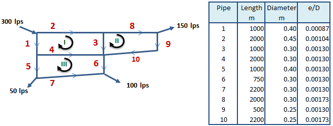
A water supply distribution system is shown in the figure below. All pipes are cast iron with lengths and diameters as provided in table below. Perform pipe network analysis and calculate water flow in all branches.

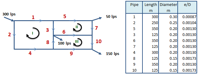
An initial flow estimate is made across all pipe branches that satisfies continuity at all nodes. Head loss across a pipe is determined using Darcy - Weisbach equation.

HLoss = K Q²
K    = 8fL/ π²g D 5

Head loss across each loop is made.

F(I)  : K1.Q1² + K3.Q3² - K8.Q8² - K4.Q4² - K2.Q2² = 0
F(II) : K5.Q5² + K7.Q7² - K6.Q6² - K3.Q3² = 0 
F(III): K6.Q6² + K10.Q10² - K9.Q9² + K8.Q8² = 0

Newton Raphson method is used to solve above equations for change in flow ΔQ (ΔQ_I, ΔQ_II, ΔQ_III) across each loop. In vector form all loops can be written as :

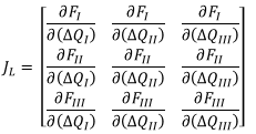
 JL.ΔQ = - F(Qm-1)
 JL    = δF / δ(ΔQ)

where Q^m-1 is vector of pipe flow, ΔQ is vector of loop flow corrections and F(Q^m-1) is the vector of residuals of loop conservation of energy equations evaluated at Q^m-1. J_L is first derivatives of the loop equations evaluated at Q^m-1. Once above matrices are formed, it is solved linearly for ΔQ and pipe flows are updated by the loop corrections as Q^m = Q^m-1 +/- ΔQ.

Coefficient Matrix, J_L

Derivative for single pipe is obtained as:

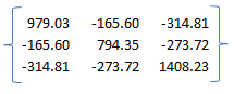
 δ(K1.Q1²)/δ(ΔQI) = 2.K1.Q1 = 2.HL1/Q1

Diagonal terms are obtained by adding derivatives of all pipes in a loop and always have a positive sign. eg.

 δFI/δ(ΔQI) = n( |HL1/Q1| + |HL3/Q3| + |HL8/Q8| + |HL4/Q4| + |HL2/Q2| )
            = 979.03

Off-diagonal terms are gradients for pipes that appear in different loops and always have a negative sign.

 δFI/δ(ΔQII) = -n( |HL3/Q3| ) = δFII/δ(ΔQI)
            = -165.60

In above derivative change in Loop I due to flow change in Loop II will be due to common pipe 3. Above gradient is also for δF_II/δ(ΔQ_I). The J_L matrix is obtained as following.

F(Q^m-1) is evaluated based on head loss across each loop.

 FI = HL1 + HL3 - HL8 - HL4 - HL2
    = -10.94

F matrix is obtained as

 F(Qm-1)T = [-10.94 -6.40 43.62 ]

Below matrix is solved in excel to obtain ΔQ.

 JL.ΔQ = - F

J_L^-1 is determined using Minverse function. Select 3x3 cells in excel and type MINVERSE(Input Array) and press CTRL+SHIFT+ENTER to evaluate inverse of matrix.

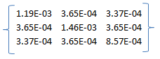
Do multiplication of J_L^-1 and -F vector using MMULT function. Select 3x1 cells in excel and type MMULT(Inverse Array, F array) and press CTRL+SHIFT+ENTER to evaluate multiplication. ΔQ array is obtained as following.

 ΔQ = [ 0.00066 -0.00261 -0.03133]

As flow changes are larger another iteration is done, with flows adjusted based on ΔQ values. For example flow rate in Pipe 3 will become.

 Q3 = Q30 + ΔQI - ΔQII
    = 0.12 + (0.00066) - (-0.00261)
    = 0.123

New flowrates are calculated and above steps are repeated. To do more iterations copy entire rows and paste them below the above cells to carry out further calculation till change in flowrates become negligible. For this example ΔQ becomes negligible in 5 iterations. Final flows in m³/s are as following.

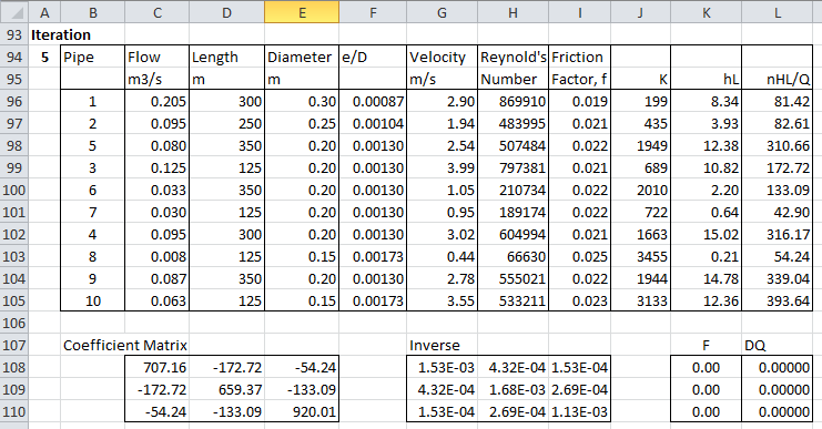
If a pipe's flow direction changes from the assumed value, the signs for that pipe head loss terms are switched for all loops containing the pipe during the next iteration in loop equations. J_L matrix signs will remain same as above.

Example

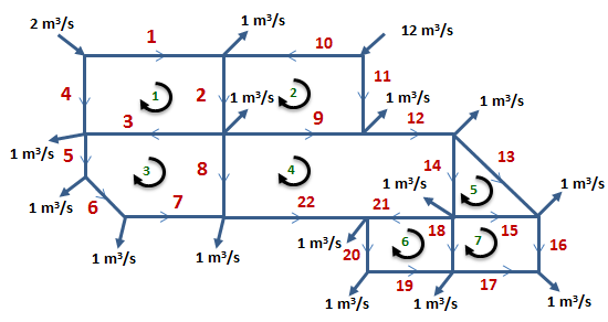
Perform pipe network analysis and calculate water flow in all branches.

This problem is solved based on methodology developed above, refer attached excel spreadsheet for solution. In this case, 3 loop equations will be made and it takes 4 iterations to converge.

Example

Perform pipe network analysis and calculate water flow in all branches. Hazen Williams coefficient for each pipe is provided in table below.

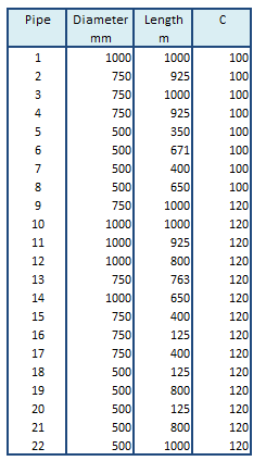
Head loss is calculated using Hazen-Williams equation.

 HL = 10.67LQ1.85 / C1.85 D4.87

Based on method discussed above 7 loop equations are formed and it takes 5 iterations to converge to final flow values. Refer attached excel spreadsheet for solution.

Resources

1. Spreadsheet for Pipe Network Analysis